In contrast to humans, neural networks tend to quickly forget previous tasks when trained on a new one (without revisiting data from previous tasks). In our recent ICPR 2018 paper we propose the rotated elastic weight consolidation (REWC) method to prevent forgetting, which builds upon elastic weight consolidation (EWC).
Sequential learning
A very common (often implicit) assumption in machine learning is that all data to learn the task(s) of interest is available beforehand. The different tasks (or the aggregated task) are learned jointly at the same time in a single training process in a multi-task fashion. The following example shows an example with three classification tasks: classifying breeds of dogs (task 1), cats (task 2) and birds (task 3), trained jointly using all the data available.
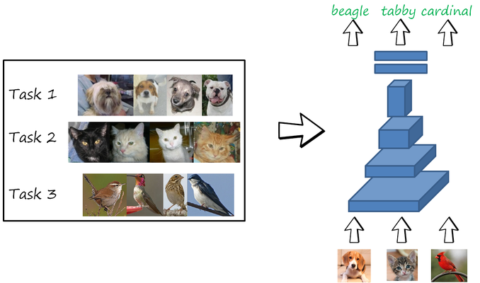
In this setting, the neural network can perform well in the three tasks. However, this is not a very realistic setting for humans, who continuously learn from the data observed during their lives, and yet can remember how to perform tasks learned in the distant past. Similarly, intelligent autonomous systems (e.g. robots, autonomous vehicles) should also be able to learn tasks in a sequential manner while remembering previously learned ones.
This problem is often referred to as lifelong learning (originally used referring to learning in humans, as the “ongoing, voluntary, and self-motivated pursuit of knowledge for either personal or professional reasons”), but other terms have been used in the literature with similar sense, such as sequential learning, continual learning or incremental learning. In my opinion, none of these terms is clear nor specific enough, and even sometimes the same term is used to refer to different settings or problems. I will use sequential learning here.
A common and controllable scenario to evaluate sequential learning is a classifier trained sequentially with a sequence of independent tasks. Each task is trained with the corresponding task-specific dataset, and data from other task-specific datasets are not available. While perhaps not completely realistic, this scenario gives a controlled setting with clearly separated tasks and where learning and forgetting can be monitored across different time steps.
The simplest baseline is sequential fine tuning, where the parameters of a network (already trained on previous tasks) are fine tuned with the data to learn the current task. For the first task, the network is typically initialized randomly. The following example illustrates this scenario, and how learning to classify cats interferes with the knowledge about classifying dogs and causes forgetting it (often known as catastrophic forgetting). Similarly, learning the bird task interferes and causes forgetting the classifying dogs and cats tasks.
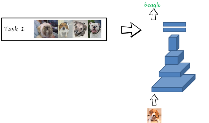
Catastrophic interference and forgetting
Joint training
A classification task is described by a dataset \mathcal{D} = \left(\mathcal{X},\mathcal{Y}\right), consisting of input values \mathcal{X}=\left ( x_1,x_2,...,x_N \right ) and the corresponding labels \mathcal{Y}=\left ( y_1,y_2,...,y_N \right ). The classification task can be described as learning the posterior probability p\left(\theta \vert \mathcal{D}\right) of the parameters \theta of the neural network given the training dataset \mathcal{D}. We can decompose it using the Bayes’ theorem and taking logarithms as
\underbrace{\log p\left(\theta \vert \mathcal{D}\right)}_{\text{posterior}}=\underbrace{\log p\left(\mathcal{D} \vert \theta \right)}_{\text{likelihood}}+\underbrace{\log p\left ( \theta \right )}_{\text{prior}}-\log p\left(\mathcal{D}\right)
A deep neural network is often trained using maximum likelihood estimation by minimizing the loss \mathcal{L}\left(\theta\right)=-\log p\left(\mathcal{D} \vert \theta \right)=-\log p\left(\mathcal{Y} \vert \mathcal{X}, \theta \right), and ignoring the prior (although there is a lot of interest in Bayesian deep learning). For classification the common choice is the cross-entropy loss (which arises from maximum likelihood estimation with a categorical distribution as likelihood).
Sequential fine tuning
Now let us imagine that the dataset \mathcal{D} is split into two disjoint sets \mathcal{D}_A and \mathcal{D}_B corresponding to task A and task B, respectively. The sequential learning problem consists of first learning task A and then learning task B (using the same network and without observing again data from task A).
The (maximum likelihood) solution for the first task \theta_A^* results from minimizing the corresponding loss with the corresponding dataset
\theta_A^*=\arg\max_\theta \mathcal{L}_A\left ( \theta \right )
Similarly, the second task is learned by continuing the training on the new task and dataset
\theta_B^*=\arg\max_\theta \mathcal{L}_B\left ( \theta ; \theta_A^*\right )
where the explicit inclusion of \theta_A^* indicates that the parameters of the network are initialized with the parameters resulting from learning the previous task.
Unfortunately this results in forgetting task A. To understand why, it is helpful to consider the following example. Imagine a very simple model with only two trainable parameters \theta_1 and \theta_2 (a particular trained model is a point \theta=\left(\theta_1,\theta_2\right) in this parameter space). The learning process for task B is represented in the following figure
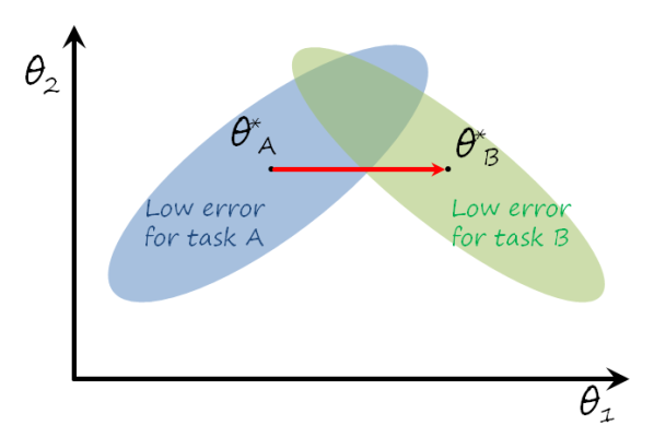
The point \theta_A^* corresponds to the specific model learned for task A, i.e. the minimum of \mathcal{L}_A\left ( \theta \right ). The region shaded in blue represents the models where the loss is still low enough for task A. We would like to stay in that region, because that means that we still remember task A. Similarly for task B and the region shaded in green. When learning task B the dynamics of gradient descent will move \theta from the initial solution \theta_A^* towards the optimal solution for task B, \theta_B^*. Since no data related with task A is observed and there is nothing that prevents from leaving the optimal area for task A, the solution after learning task B will likely forget task A. Ideally, we would like to stay in the intersection between the two shaded areas, since that would correspond to remembering both tasks. There is always a compromise between learning task B and remembering task A, since all parameters are shared by both tasks, and optimizing for task B will move \theta away from the optimal solution for task A, in other words, there is an interference between both tasks, that results in the catastrophic forgetting of task A.
Preventing forgetting. As we just saw, catastrophic forgetting arises naturally when neural networks are trained in a sequential learning setting simply using fine tuning. There have been numerous efforts to devise other network architectures and training algorithms that can prevent or at least alleviate catastrophic forgetting. Roughly speaking, there are three type of approaches to prevent forgetting:
- Rehearsal and pseudorehearsal. Observing training data of a particular task is what guides the gradient to low error regions for that tasks. Rehearsal methods relax the sequential learning constraints to allow a memory with a few samples from previous tasks (a.k.a exemplars) that are revisited while learning new tasks effectively prevents forgetting (e.g. the exemplars from task A would bias the gradient back to the blue region). In a strict sequential learning setting without exemplars, it is possible to learn a generative model of the samples of previous tasks. While learning new tasks, pseudosamples are sampled and used in a similar way (i.e. pseudorehearsal).
- Regularization. The absence of any constrain . These methods are based on preventing weights or activation from changing significantly from the ones obtained in previous range.
- Develop modularity. Using the same weights between tasks causes interference and consequently forgetting. Some methods prevent this interference by implicitly or explicitly forcing different tasks to use different sets of parameters (e.g. imagine that in the example the solution for task A only depends on \theta_1, and for task B only on \theta_2, then learning task B would not interfere with remembering task A). In the extreme case you can train separate networks for each task, but this can be also not optimal, since you would not exploit potential benefits of sharing representations and reusing knowledge from similar tasks.
Elastic weight consolidation
We focus now on elastic weight consolidation (EWC), which prevents forgetting by regularizing the weights.
Intuition. We can grasp the idea behind EWC revisiting the previous two tasks example. The following figure shows a more ideal learning trajectory that leads to a solution with low error in both tasks.
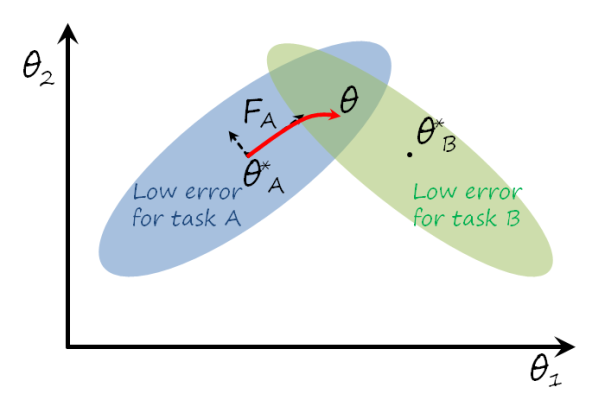
Two observations:
- The further \theta moves away from \theta_A^*, the more likely is to forget task A. This suggests that penalizing the distance between \theta and \theta_A^* can help to keep the solution in the blue region.
- Some directions are more prone to forgetting than others. For instance, in the example, moving northwest or southeast forgets much faster that moving northeast or southwest. Therefore the latter directions are safer if we want to prevent forgetting task A.
EWC tries to keep the gradient descent in a safe trajectory by penalizing the distance to the solution for previous tasks, with less penalty on safer directions.
Bayesian perspective. In the paper the authors use a Bayesian formulation, where previous tasks are considered as priors of the current task. In the two tasks example, the objective after learning task B should optimize the joint posterior \log p\left(\theta \vert \mathcal{D_{AB}}\right), where \mathcal{D}_{AB} is the combined dataset of both tasks. Using the Bayes’ theorem again, we obtain
\underbrace{\log p\left(\theta \vert \mathcal{D_{AB}}\right)}_{\text{posterior (both tasks)}}=\underbrace{\log p\left(\mathcal{D_B} \vert \mathcal{D_A}, \theta \right)}_{\text{likelihood (current task B)}}+\underbrace{\log p\left ( \theta \vert \mathcal{D_A}\right )}_{\text{prior (solution of task A)}}-\log p\left(\mathcal{D_B} \vert \mathcal{D_A}\right)If we again assume that \mathcal{D_A} and \mathcal{D_B} are independent, we obtain
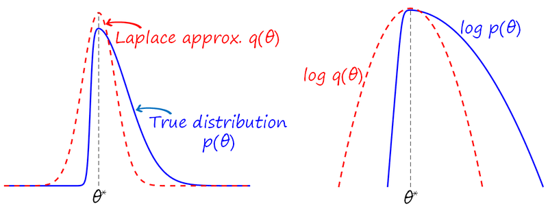
\log p\left(\theta \vert \mathcal{D_{AB}}\right) = \log p\left(\mathcal{D_B} \vert \theta \right)+\log p\left ( \theta \vert \mathcal{D_A}\right )-\log p\left(\mathcal{D_B}\right) The first term of the right-hand side corresponds to the conventional loss for task B (i.e. maximum likelihood over \mathcal{D_B}). The second term is the prior for task B, corresponding to the posterior of task A. Since this posterior is intractable, EWC uses the Laplace approximation.Laplace approximation. After training a neural network we obtain a single value \theta^* that maximizes a log-likelihood \log p\left ( \theta\right ). In the Laplace approximation, the true distribution p\left(\theta\right) is approximated in the proximity of \theta^* by a Normal distribution q\left(\theta\right)={\mathcal {N}}(\theta \vert\mu ,\Sigma) (see the figure below). The mean of this Normal distribution is set to \theta^* and the covariance matrix is estimated as the inverse of the Fisher information matrix (FIM).
Back to our example, applying the Laplace approximation for task A and taking logarithms, the log-prior for task B becomes the quadratic form \log p\left ( \theta \vert \mathcal{D_A}\right ) \approx -\frac{1}{2}\left( \theta - \theta_A^* \right)^\intercal F_A \left( \theta - \theta_A^* \right) + C
and the joint posterior becomes
\log p\left(\theta \vert \mathcal{D_{AB}}\right) \approx \log p\left(\mathcal{D_B}\vert \theta \right)-\frac{\lambda}{2}\left( \theta - \theta_A^* \right)^\intercal F_A \left( \theta - \theta_A^* \right) + C'
where \lambda is a hyperparameter introduced to trade off learning task B and not forgetting task A.
Computing the Fisher information matrix. The FIM of the log-likelihood for task A at the maximum \theta_A^* observing the dataset \mathcal{D}_A is
F_A = \left.\mathbb{E}_{\mathcal{D}_A}\left[\left (\frac{\partial \log p\left(\mathcal{D}_A\vert \theta \right )}{\partial \theta}\right)\left(\frac{\partial \log p\left(\mathcal{D}_A\vert \theta \right )}{\partial \theta}\right )^{\intercal}\right]\right |_{\theta=\theta_A^*}
The FIM also corresponds to the Hessian of the log-likelihood, i.e. F_A = \left.\mathbb{E}_{\mathcal{D}_A}\left[\frac{\partial^2 \log p\left(\mathcal{D}_A\vert \theta \right )}{\partial \theta^2}\right]\right |_{\theta=\theta_A^*}, which estimates how fast we may forget task A depending on the direction. The EWC regularization term encourages moving in directions with low Fisher information.
Limitations and diagonal approximation. For a model with N parameters, the FIM has a size of N^2, which is impractical for medium size networks with tens of thousands or million parameters. Estimating such amount of parameters is also problematic with the limited data available. Therefore, the FIM in the Laplace approximation is often assumed to be diagonal, which only requires N parameters (an additional reason is that inverting a diagonal matrix is much easier and cheaper, which is required in many problems although not in our case). EWC also uses a diagonal FIM.
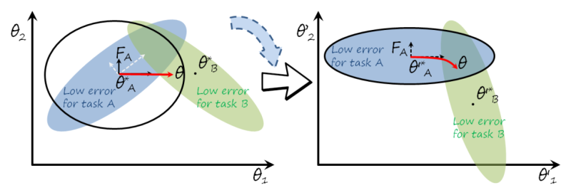
However, the diagonal approximation implies the assumption that perturbations in one parameter do not affect the other parameters (which is obviously not true), and makes the FIM ignore the correlation between dimensions in the parameter space. The following figure illustrates that case, where the contours obtained with the diagonal approximation (black ellipse) may differ significantly from the contours estimated with the full FIM (blue shaded ellipse), leading to suboptimal trajectories with more forgetting. Note how the axes of the black ellipse are aligned with \theta_1 and \theta_2.
Rotated elastic weight consolidation
The main idea in rotated elastic weight consolidation (R-EWC) is to rotate the parameter space in such a way that the diagonal approximation of the FIM is a good approximation of the full FIM, and then learn task B in that rotated space (see previous figure).
Now the question is how to implement such rotation. In fact, such rotation is probably impossible to implement in a feed-forward neural network without breaking it. We propose the following approximation. First we apply rotations layerwise (i.e. each layer independently). Then we approximate each rotation with additional layers that will rotate the input and the output of that layer.
Rotating fully connected layers. For simplicity, we first consider the case of a single fully-connected layer given by the linear model \mathbf{y}=W\mathbf{x}, with input \mathbf{x} \in \mathbb{R}^{d_1}, output \mathbf{y} \in \mathbb{R}^{d_2} and weight matrix W\in \mathbb{R}^{d_2 \times d_1}. In this case \theta=W, and to simplify the notation we use L=\log p\left(\mathbf{y}\vert\mathbf{x};W\right). The FIM in this simple linear case is (after applying the chain rule):
F_W = \mathbb{E}_{\mathbf{x}\sim \pi, \mathbf{y}=p\left(\mathbf{y}\vert\mathbf{x};W\right) }\left[\left (\frac{\partial L}{\partial \mathbf{y}}\frac{\partial \mathbf{y}}{\partial W}\right ) \left(\frac{\partial L}{\partial \mathbf{y}} \frac{\partial \mathbf{y}}{\partial W}\right )^{\intercal} \right]=\mathbb{E}_{\mathbf{x}\sim \pi, \mathbf{y}=p\left(\mathbf{y}\vert\mathbf{x};W\right)}\left[\left (\frac{\partial L}{\partial \mathbf{y}}\right) \mathbf{x}\mathbf{x}^{\intercal} \left (\frac{\partial L}{\partial \mathbf{y}}\right )^{\intercal} \right]
where \pi is the empirical distribution of input features \mathbf{x} to the layer. If we further assume that \frac{\partial L}{\partial \mathbf{y}} and \mathbf{x} are independent random variables we can factorize F_W as
F_W=\mathbb{E}_{\mathbf{x}\sim \pi, \mathbf{y}=p\left(\mathbf{y}\vert\mathbf{x};W\right)}\left[\left (\frac{\partial L}{\partial \mathbf{y}}\right) \left (\frac{\partial L}{\partial \mathbf{y}}\right )^{\intercal}\right] \mathbb{E}_{\mathbf{x}\sim \pi}\left[ \mathbf{x}\mathbf{x}^{\intercal} \right]
Note that now one of the factors in this approximation depends on the input features and the other in the backpropagated gradients at the output. Now we can apply two singular value decompositions (SVD) on each of the factors to obtain
\mathbb{E}_{\mathbf{x}\sim \pi, \mathbf{y}=p\left(\mathbf{y}\vert\mathbf{x};W\right)}\left[\left (\frac{\partial L}{\partial \mathbf{y}}\right) \left (\frac{\partial L}{\partial \mathbf{y}}\right )^{\intercal}\right]=U_2 S_2 V_2^{\intercal}
\mathbb{E}_{\mathbf{x}\sim \pi}\left[ \mathbf{x}\mathbf{x}^{\intercal} \right]=U_1 S_1 V_1^{\intercal}
where U_1 and U_2 can be seen as rotations of the input and output of the linear layer. This can be implemented as two additional linear layers whose weights are learned first after training task A using the previous equations, and then fixed. Task B is then trained over the new problem \mathbf{y}'=W'\mathbf{x}'. The following figure illustrates the implementation in a neural network
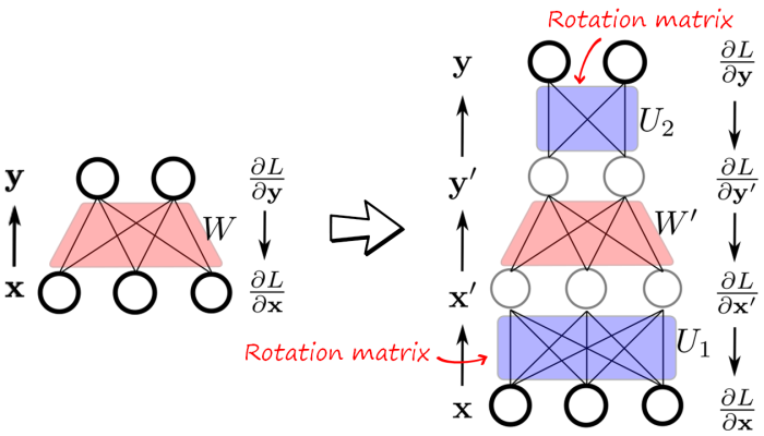
Note that the forward passes in the original network (left) and the rotated network (right) are equivalent, since W'=U_2^\intercal W U_1^\intercal.
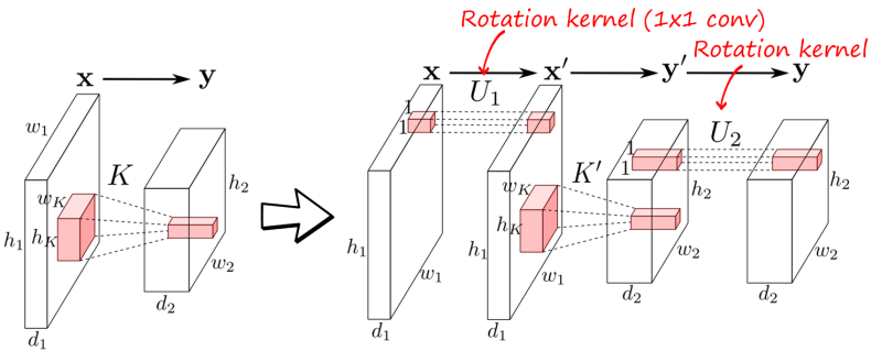
Rotating convolutional layers. The same idea can be applied to convolutional layers using 1×1 convolution kernels, as shown in the following figure
To illustrate the effect of this rotation, the following figure shows the fully FIM of a fully connected layer in a toy neural network (left), the rotation using SVD in the parameter space (center), which is not possible in practice, and the result of the indirect rotation in R-EWC (right).
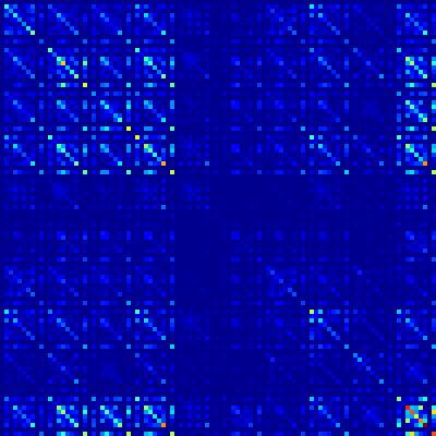
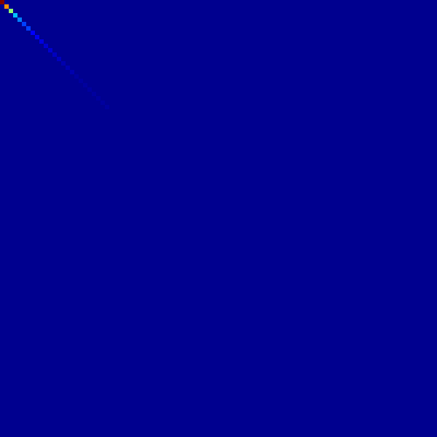

Remember that we always use the diagonal approximation to learn the new task B. The diagonal in the orginal FIM in the example contains 40% of the energy, while in the rotated version with our method contains 74%, meaning that the diagonal approximation after rotation keeps more information.
Results
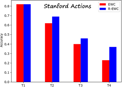
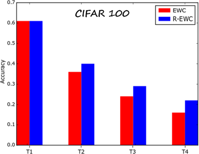
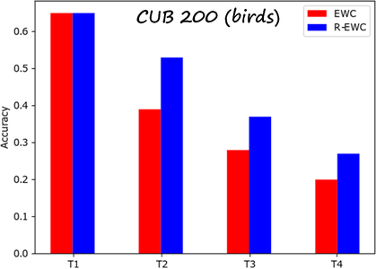
We compared R-EWC and EWC on several datasets. The following results are computed on a sequence of four tasks (each dataset is split into four subsets with equal number of classes). The metric is the average accuracy over all tasks learned so far. The datasets are Stanford Actions, CIFAR-100 and CUB-200 (fine-grained bird classification). The results show that the R-EWC can prevent forgetting previous tasks better than EWC.
